Last time, we looked at how to organize your OpenSCAD code. This time, we’ll get a little bit more advanced. We’re going to make cookie cutters! And in the process, we’ll learn about linear extrusion, Minkowski Sum, and how to do offsets in OpenSCAD.
Let’s say it’s Christmas time, and you want to make your honey happy. She loves chess and you decide to make her some knight-shaped cookie cutters. But your local Crate and Barrel (a home goods store in the US) isn’t going to carry such specialized cookie cutters.
Time to roll up your sleeves and make your own.
First, we make an outline of a knight profile in any vector drawing program that exports to DXF, like Inkscape. I won’t cover that process here, since it’s beyond the scope of this guide, but you can download a pre-made one here (just click the download button).
However, note that if you decide to draw your own DXF file, you’ll need to install a plugin for Inkscape that will export to a DXF format. Once we have our DXF file, we can import it into OpenSCAD pretty easily with the import function.
import(file="knight_profile.dxf");Notice here that it’s still a 2D shape. In order to make it a 3D shape, we’re going to extrude it vertically. Linear extrude is like stretching and projecting a shape in the z-direction. It gets its name from the mechanical process of making a long shape with the same cross-sectional profile.
In OpenSCAD, this is also pretty easy. Linear extrude has many more options, but the important one to pay attention to is the height. It dictates how far off the XY-plane we should extrude. We’ll wrap it all in a module called knight_profile().
module knight_profile() {
  linear_extrude(height = 5)
    import(file="knight_profile.dxf");
}
Now that we have a 3D extrusion, it’s still not usable as a cookie cutter, as there’s no actual hole to cut out our cookie. At best, we merely have a stamp. So our task now is to punch a hole with the exact same outline, but smaller inside of our knight-shaped extrusion.
Offset
What we need is called an “offset” in other types of CAD packages. We would like an expanded outline of our extruded shape. When we’d like a shrunken outline of our extruded shape, it’s called an inset.

We can see here that on the left is the original extruded shape. The middle is the offset shell. The right-most shape is the inset shell.
Well, there’s no OpenSCAD function called offset or inset. What to do? We build our own from OpenSCAD’s primitives! This is what I meant by building abstractions, where we can think about manipulating our model at a higher level.
One way we could do this is to find the center of mass of our shape, and then scale the knight in the X and Y direction, then difference that shape. However, calculating the center of mass is not easy for arbitrary shapes, and only done for the simplest of shapes. In addition, that method wouldn’t work for concave shapes.
Building offset with the Minkowski Sum
The secret to building offset is to use the Minkowski Sum! But what’s a Minkowski Sum? That bears a bit of explaining. The Minkowski sum is a way to integrate two shapes together, by using the second shape to trace the surface of the first, and union-ing all the places the second shape had been while tracing.
Example time! If we look at an example of applying Minkowski to a Square and a Circle, we can see that when we imagine using the circle as a “pen”, and tracing the outline of the square.

When we look at the unioned result, we get a rounded square. That is our Minkowski Sum in two dimensions.

In three dimensions, when we apply the Minkowski Sum to a cube and a sphere, we can imagine the sphere as a “pen”, and tracing the surface of the cube.

When we look at the resulting Minkowski, we get a cube with rounded corners.

Note that the minkowski sum is commutative, meaning it doesn’t matter if you think of the square or circle as the “pen” doing the tracing. The resulting sum is the same.
By now, you should realize that an offset is just the minkowski sum of our extruded knight profile with a cube! And then to get our cookie cutter, we can difference the offset with the original extrusion. Note that we didn’t need to calculate the center of mass, and this works on any arbitrary shape, translated anywhere in space. So let’s code it up!
module knight_profile() {
linear_extrude(height = 5)
import(file = "knight_profile.dxf");
}
difference() {
render() {
minkowski() {
knight_profile();
cube(center=true);
}
}
translate([0, 0, -1]) scale([1, 1, 1.5])
knight_profile();
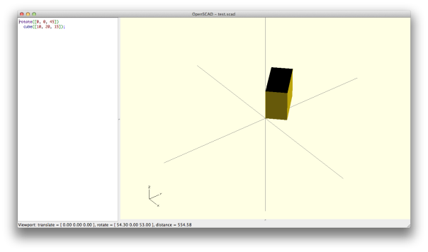
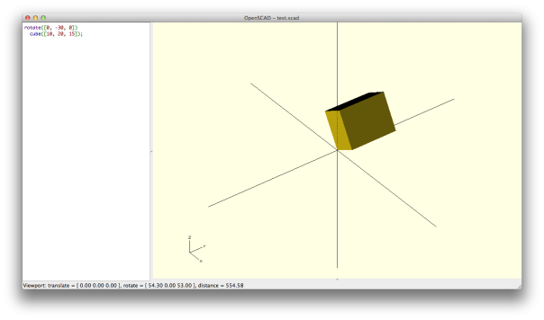
}Now, the Minkowski can take a long time to compute. As such, that’s why we used a cube, so there’s as little faces to process as possible while tracing the original shape. In addition, you can wrap the minkowski() in a render(), to cache the results, so OpenSCAD doesn’t have to compute it every time something changes in the file, outside of the render() block.
Lastly, we scale the knight extrusion by 1.5 in the z direction and then translate it by -1 to get rid of co-incident planes that results in shimmering. And we now get the offset shell of the knight!

Making our solution reusable
However, our solution isn’t reusable, let’s put it in a module called offset_shell() that takes a single parameter controlling the thickness of the offset.
module offset_shell(thickness = 0.5) {
  difference() {
    render() {
      minkowski() {
        children();
        cube([2 * thickness, 2 * thickness, 2 * thickness], center=true);
      }
    }
    translate([0, 0, -5 * thickness]) scale([1, 1, 100])
      children();
  }
}
Note the biggest changes are the adjustments to the thickness of the offset, and the use of the children() function, which allow us to operate on modules nested within offset_shell(). And we can use it like so:
offset_shell(1)
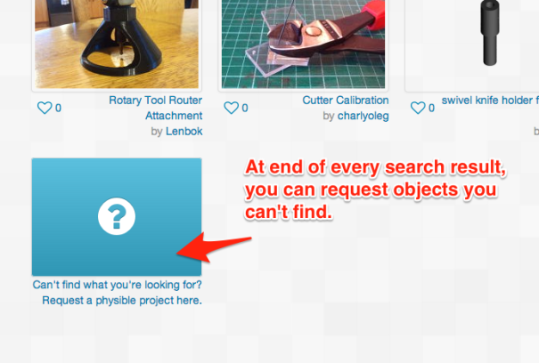
knight_profile();Whenever you see children() in the code, it refers to the resulting shape of the children of offset_shell(). In this case, it refers to the knight_profile(). Instead of writing it yourself, I’ve put it up in a library on Cubehero, so you can use it yourself.
The library’s README.md has more explicit and up to date instructions on how to use it. Now our offset is abstracted, and we don’t have to worry about any of the details again!
Insets
So what about insets? That is a little trickier, as there’s no Minkowski Subtraction operation–akin to using the second shape to cut from the first shape while tracing the surface first shape. However, there’s a trick we can employ. First, we can invert our knight_profile (turn it inside out), by differencing a very large cube with our extruded knight_profile.
When you run the code below, you won’t see the picture the follows. But I faked it so you can get a sense of what it’s doing. I show a smaller transparent cube here in the picture for illustrative purposes. The red signifies a hole.
module invert(bbox = [5000, 5000, 5000]) {
  difference() {
    cube(bbox, true);
    children();
  }
}

invert() knight_profile();

So we get a huge cube with a knight_profile shaped cave inside of it. If we run the Minkowski on that, we’d get the shape of the inverted inset! That’s because the minkowski traces the entire surface, regardless of whether it’s on the outside or inside.
minkowski() {
  invert() knight_profile();
  cube([1, 1, 1], center=true);
}
Now that we have the inverted inset, we want the inset. To get the inset however, we now need to turn the inverted inset right-side out. We can do that by subtracting the inverted inset from a smaller bounding box.
invert(0.9 * bbox)
  minkowski() {
    invert() knight_profile();
    cube([1, 1, 1], center=true);
  }
And now, to get the inset shell, we cut the inset shape from the original extruded knight, by expanding it in the z direction and shifting it downwards to make sure there aren’t any co-planar surfaces. Again, the inset is represented in red as a hole.
difference() {
  children();
  translate([0, 0, -5]) scale([1, 1, 100])
    translate([0, 0, -2])
      invert(0.9 * bbox)
        minkowski() {
          invert() knight_profile();
          cube([1, 1, 1], center=true);
        }
}
 Now, we’ll refactor it all so that it’s readable, and useable without worry about the low-level details:
module inset_shell(thickness = 0.5, bbox = [5000, 5000, 5000]) {
  module invert(bbox = [5000, 5000, 5000]) {
    difference() {
      cube(bbox, true);
      children();
    }
  }

  module inset(thickness = 0.5, bbox = [5000, 5000, 5000]) {
    render() {
      invert(0.9 * bbox)
        minkowski() {
          invert() children();
          cube([2 * thickness, 2 * thickness, 2 * thickness], center=true);
        }
    }
  }

  render() {
    difference() {
      children();
      translate([0, 0, -5 * thickness]) scale([1, 1, 100]) translate([0, 0, -2 * thickness])
        inset(thickness, bbox)
          children();
    }
  }
}

inset_shell(1)
  knight();
Again, you don’t have to write everything yourself. I’ve wrapped it all in a library for you to use. A couple things to notice:
First, by default, this only works with shapes that are smaller than 5000x5000x5000. In OpenSCAD, there isn’t an easy and fast way to programmatically the bounding box of a shape. (It does exist, but it’s damn slow). That’s why we allow the user to change the default size on the bounding box. But most of the time, the default will work nicely and won’t need to be specified.
Second, we wrap the inset shell with a render, because otherwise the result won’t render correctly on the screen. OpenSCAD takes shortcuts to render CSG results fast (when you render with F5), but there are edge cases where it doesn’t work and you need to do the full CSG computation (when you render with F6).
Lastly, modules can be nested. The invert module and inset module is nested inside of the inset_shell module. That means modules outside of inset cannot use invert or inset. But in this case, we use it to make our code more readable.
For the more astute amongst you, you may have noticed you can skip the second inversion step and just intersect the inverted inset with the original extrusion to get the inset shell. And you’d be right! But I couldn’t get it to work with different inset thicknesses. If you have patches to submit, I’d be happy to incorporate it. Make sure you try it with different thicknesses from 0.1 to 20.
In Summary
Now your honey is happy with her chess pieces, and you find some other way to make the holidays bright. Offsets and insets are easy to do in OpenSCAD once you know about the Minkowski Sum. The library for offsets from this blog post is hosted on Cubehero.
Let me know that you find these helpful by signing up for my mailing list to get more OpenSCAD guides as I write them. It’ll motivate me to write more! See what I’ve written previously on OpenSCAD. If you’d like to see what else I work on, check out Cubehero, or follow me on twitter.